The most recent JLL viz challenge had the theme “White Space”, based on the recent Iron Quest challenge of the same name. Since the theme focused on design aspects of dataviz, I went looking for data sets in design’s cousin field: fine art.
I went searching for artists known for their use of white space or negative space - that design concept that uses unmarked space between design elements to act as another design element in itself. And what I found was conceptual artist Sol LeWitt and his 1974 work “Incomplete Open Cubes”. Or rather, I found a really excellent article about the work, called “‘Irrational Thoughts Should be Followed Absolutely and Logically’: Sol LeWitt’s ‘Variations of Incomplete Open Cubes’ (1974)” by Mariabruni Fabrizi. I became quickly infatuated with recreating LeWitt’s cubes (and maybe also proving to myself that his series was complete).
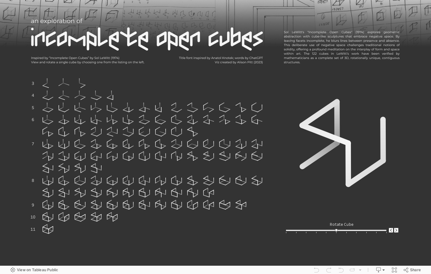
LeWitt’s piece describes 122 configurations of what is essentially a wireframe cube with one or more edges removed. While each configuration is “incomplete”, the space between the edges left over implies the same cube shape. LeWitt created the piece manually, but it’s since been confirmed by mathematicians to be a complete set of all possible configurations.
Click here to view the completed viz on Tableau Public, or read on for more details.
This video from the San Francisco Museum of Modern Art has some additional context:
Determining the cubes
To my knowledge, attempting to determine LeWitt’s cubes using a data (ETL) focused approach has not been done before. For this part of the exercise, I used Alteryx to do the heavy lifting. This is admittedly a brute-force method (other mathematical approaches use graph theory), but it works.
To start, I decided I would define a cube frame, find all possible “incomplete cubes” and then eliminate invalid configurations. The first part was easy: a cube has 6 faces, 8 vertices and 12 edges. If I defined each edge and worked out all possible combinations, that’s 4095 - well, 4094, since one of those combinations is a complete cube.
For this part, I defined a 1x1x1 cube with one vertex at (0,0,0) and the rest of the cube in the positive-xyz space. I named the edges A-L and used a 12-digit binary number to define the possible configurations; each bit on/off would correspond to an edge included or excluded from the configuration.

The drawing I used to keep track of the edges and vertices in my cube model
Once I had all the possible configurations, it was time to eliminate invalid ones.
Eliminating invalid cubes
In my reading, I found “Incomplete Cubes Revisited” by Rob Weychert. The author helpfully enumerated the criteria for including a configuration in the final list of 122:
Dimensionality: does a configuration describe three dimensions?
Contiguity: does each edge touch at least one other edge?
Rotation: is a configuration unique, rotationally?
Dimensionality was the simplest, so I tackled that first.
Dimensionality
If the difference between min and max coordinates in each dimension of a configuration is 1 (on the cube as described), then a configuration describes three dimensions.
In Alteryx, I brought in the coordinates of each edge, calculated the mins and maxes, and eliminated configurations where the min-max was 0 in any dimension.
Rotation
Rotation and contiguity were the two criteria that I expected to be the toughest (spoiler: I was right). So I looked at rotation first, since I thought it had the potential to eliminate the most invalid configurations (I did not go back to test whether this assumption was true).
To test for rotationally-unique configurations, I first defined all the ways that a given configuration could be rotated. From a given starting point, a cube can be rotated up to three times in any dimension. That means that every configuration could have up to 256 rotationally-equivalent variations in the list of 4,094.
(Now, this next part is probably the least-effective way to determine which configurations are rotationally-equivalent, but I would maintain that it’s probably the coolest.)
To work out the rotational variations of each configuration, I created ciphers that described the progression of edges as they are turned in each dimension:
x: AIKC, BFJG, DELH
y: DLJB, CHKG, EIFA
z: ABCD, EFGH, IJKL
I applied these ciphers to all the possible rotations of all the configurations, then eliminated duplicates.
Contiguity
Contiguity actually ended up being the most difficult criteria to understand. I tried a few different methods before settling on this one: I created an Alteryx macro that would traverse every possible contiguous path from every possible starting edge, and if the set of contiguous edges described by the paths matched the overall configuration, then the configuration was valid.
Since this method generated a lot of paths, I did do one step before heading into the macro: I pre-eliminated any configurations where there was one or more edges with no adjacent edges.
After I applied the dimensionality, rotation and contiguity criteria to the original list of 4,094 configurations, I was left with exactly 122 configurations, the same as LeWitt’s.
Next, I brought the cubes into Tableau for visualization.
Visualizing the cubes
In order to create the cube drawings in Tableau, I knew I would want a “line” type chart, which needs the points to draw, plus the order in which to draw them. I decided it would be too hard to draw full shapes, so I opted to draw edges instead. I structured the data to have unique rows for the start and end of each edge in each configuration, with the field [Path Order] defining the ends.
But…how do you visualize a three-dimensional object in a two-dimensional application like Tableau?
Showing 3D objects in 2D
I found inspiration from Bora Beran’s excellent “Going 3D with Tableau” blog post. I didn’t end up using their method, but it did point me to the Wikipedia page for rotation matrices, which I did use.
For my methodology, I used two facts:
You can project a 3D object onto the xy plane in Tableau simply by omitting the z-coordinates.
You can use a rotation matrix to rotate a 3D object in 3D space.
From here, I generated my charts in three steps:
Translated my cubes to be centered on (0, 0, 0). For simplicity in calculating the cubes I had defined my original coordinates as centered on (0.5, 0.5, 0.5). Translating to (0, 0, 0) is just a matter of subtracting 0.5 from each (x, y, z).
Applied a 3D rotation matrix to each (x, y, z).
Created a line chart for each configuration, using the rotated x value on columns, rotated y value on rows, edge on detail on the marks card, and path order on path.
The 3D rotation matrix is really the key here. It looks really scary, but it’s just a way of describing the calculations you need to use. Wikipedia has the definitions for translating 3D points according to yaw, pitch and roll angles:
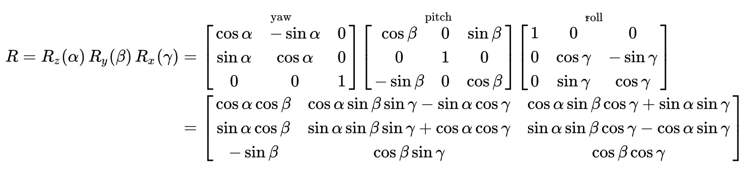
A general 3D rotation matrix, from Wikipedia
In Tableau, this looks like (with parameters for yaw, pitch and roll angles):
[x_r] =[X_centered] * (COS([Yaw]) * COS([Pitch]))+ [Y_centered] * (COS([Yaw]) * SIN([Pitch]) * SIN([Roll]) - SIN([Yaw]) * COS([Roll]))+ [Z_centered] * (SIN([Yaw]) * SIN([Roll]) + COS([Yaw]) * SIN([Pitch]) * COS([Roll]))
[y_r] =[X_centered] * (SIN([Yaw]) * COS([Pitch]))+ [Y_centered] * (COS([Yaw]) * COS([Roll]) + SIN([Yaw]) * SIN([Pitch]) * SIN([Roll]))+ [Z_centered] * (SIN([Yaw]) * SIN([Pitch]) * COS([Roll]) - COS([Yaw]) * SIN([Roll]))
[z_r] =[X_centered] * (-1 * SIN([Pitch]))+ [Y_centered] * (COS([Pitch]) * SIN([Roll]))+ [Z_centered] * (COS([Pitch]) * COS([Roll]))
Once the line chart was set up, then I tweaked the appearance of the cube by modifying the yaw, pitch and roll angles (each ranging from 0 to 2 pi).
Giving the cubes depth
I used three “tricks” to make the cubes appear to have depth in 2D:
I added color to delineate “near” from “far” points.
I ensured that “near” edges were drawn last, and therefore on the top of the chart.
I created a secondary rotational matrix to allow users to “rotate” the cube in a limited way.
Since in Tableau we’re effectively viewing the xy plane from the top down, I applied a custom sequential color on the rotated z coordinate, with negative z-values being a darker color than positive. (Incidentally this the opposite from a typical teaching of “atmospheric perspective”, which recommends darker colors for near objects. But since LeWitt’s original cubes were white, I made an aesthetic choice.)
As for the drawing order, I got lucky: the way I originally defined the cube, the edges went more or less alphabetically in one direction. So I just sorted edge in reverse alphabetical order (insert winky smiley face here).
For the final trick - letting users rotate the cube - I ended up doing the rotation twice: once to define a “default” rotation, and a second time with a limited-range pitch angle that users can control on the dashboard. Not a true 3D rotation, but an approximation.
Other design considerations
I created the background graphic for my dashboard in Figma. Along with the text elements, I used clips of LeWitt’s hand-drawn incomplete cubes to give it some additional interest.
For the title, I recreated the letters from a post by Anatol Knotek on Tumblr, which was also inspired by Sol LeWitt’s “Incomplete Open Cubes”.
In Tableau, I used a couple quality-of-life tricks to prevent highlighting on the cube selection chart, and to self-deselect selected edges (because they looked weird):